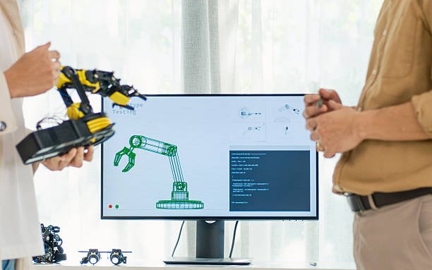
When you are working with a system that is difficult, expensive, or time-consuming to test in the real world, simulation can save a lot of effort. Instead of changing a physical setup every time you want to test an idea, you can build a mathematical representation of the system and see how it behaves on a computer.

That is where MATLAB becomes useful.

I use MATLAB as a bridge between the mathematics behind a problem and the results I actually want to see. You can use it to solve equations, work with experimental data, test different parameters, create graphs, and investigate how a system responds to changing conditions. When a problem involves several connected components or a more visual representation of a dynamic system, Simulink adds a block-diagram approach to the same workflow.

The important thing, though, is not simply getting MATLAB to produce a graph. A simulation is only useful when the model behind it makes sense and the results have been properly checked.

What does modelling and simulation mean in MATLAB?

Modelling is the process of representing a real system mathematically.

Imagine you want to study a vehicle suspension. You might represent the suspension using masses, springs, dampers and forces. Each part can be described using equations, and those equations can then be used to predict how the suspension will move when the vehicle encounters a bump.

Simulation takes that model and calculates what happens over time.

The same basic idea works for electrical circuits, motors, aircraft, chemical processes, control systems, thermal systems and many other applications.

MATLAB is particularly useful when the model can be described using mathematical equations or numerical relationships. Simulink takes the idea further by allowing you to represent algorithms and physical systems as connected blocks. It supports both linear and nonlinear systems and allows complex models to be organised into subsystems.

MATLAB or Simulink: which one should you use?

This is one of the first decisions you’ll make.

MATLAB is usually the better starting point when you need to perform calculations, manipulate data, solve equations or write a repeatable analysis script. You can keep your parameters, calculations and plots together in one file and rerun the entire analysis whenever your data changes.

Simulink is more useful when the system is easier to understand as a collection of connected components.

For example, a simple control system could contain a reference signal, controller, plant, feedback loop and output. Drawing those relationships as blocks can be much easier to follow than representing everything in a long MATLAB script.

You can also combine the two. Simulink is integrated with MATLAB, so MATLAB algorithms can be used within models and simulation results can be brought back into MATLAB for further analysis.

In practice, the choice often looks like this:

• MATLAB: equations, numerical calculations, data analysis and visualisation.
• Simulink: block diagrams, dynamic systems, feedback and system-level simulation.
• MATLAB + Simulink: larger projects where mathematical analysis and graphical system modelling need to work together.

How to build a MATLAB simulation

A reliable simulation normally starts with the problem, not the software.

Before writing code, decide what you are actually trying to find out. Once that is clear, the rest of the modelling process becomes much easier.

1. Define the problem

Start by describing the real system in ordinary language.

Suppose you want to know how the position of an object changes after a force is applied. You need to identify the quantities involved, including the input force, mass, position, velocity and time.

You should also decide what you want from the simulation.

Perhaps you need the position at a particular time. Maybe you want to see the complete response over ten seconds. Or perhaps your real objective is to determine which parameter has the greatest effect on the result.

These are different questions, and they can require different models.

2. Turn the problem into equations

Once you understand the system, express its behaviour mathematically.

For a simple mass-spring-damper system, for example, the governing equation can be written as:

md2xdt2+cdxdt+kx=F(t)

Here, m is the mass, c is the damping coefficient, k is the spring stiffness, and F(t) is the applied force.

MATLAB can solve this type of differential equation numerically.

The following example uses ode45:

m = 1;
c = 0.5;
k = 10;
model = @(t,x) [x(2);
 (1 - c*x(2) - k*x(1))/m];
[t,x] = ode45(model,[0 10],[0 0]);
plot(t,x(:,1),'LineWidth',1.5)
xlabel('Time (s)')
ylabel('Displacement (m)')
grid on

The ode45 function is designed for solving many ordinary differential equation problems that are not stiff. MATLAB provides several other ODE solvers, so ode45 should not be treated as the correct choice for every problem.

The code is relatively short, but there is an important lesson here: MATLAB cannot fix an incorrect mathematical model. If the assumptions or equations are wrong, the simulation can still produce a perfectly convincing-looking result.

3. Enter your parameters carefully

Next, define the values used by the model.

For example:

mass = 1.5;
damping = 0.8;
stiffness = 12;

Keeping these values as named variables makes your model easier to understand and modify.

It also makes parameter studies much simpler later. Instead of searching through your code for every occurrence of a number, you can change one variable and run the simulation again.

I also recommend recording the units alongside your parameters. Mixing metres with millimetres or seconds with milliseconds is an easy way to produce incorrect results without triggering a MATLAB error.

Choosing the right solver

Solver selection becomes more important as your model becomes more complicated.

A numerical solver essentially works out an approximate solution to the equations over a series of time steps. In Simulink, you can choose from fixed-step and variable-step solvers depending on the type of simulation you’re running.

A variable-step solver can adjust the time step during a simulation according to the behaviour of the model. Fixed-step approaches, meanwhile, use a specified step size and can be particularly relevant when you are considering implementation on hardware or working with discrete systems.

Don’t automatically assume that a smaller time step means your simulation is better.

A very small step can increase computation time without giving you a meaningful improvement in the answer. Instead, compare results at different settings and determine whether the change is significant for the purpose of your study.

Creating a model in Simulink

If your system contains several interacting parts, Simulink can make the model considerably easier to understand.

You create a model by placing blocks into the Simulink Editor and connecting them with signal lines. The blocks can represent mathematical operations, system components, inputs, outputs and other functions.

A basic control-system model might contain:

1. An input or reference signal.
2. A controller.
3. A model of the physical system.
4. Feedback from the output.
5. A display or logging mechanism for the results.

You can then run the model and observe how the output changes over time.

Simulink also allows related blocks to be grouped into subsystems. This becomes increasingly important when a model grows because a single diagram containing hundreds of blocks quickly becomes difficult to maintain.

One useful approach is to keep the model at a high level and place complicated sections inside clearly named subsystems. That way, you can understand the overall system without losing access to the underlying detail.

Working with real experimental data

A simulation becomes much more valuable when you can compare it with something that actually happened.

Suppose you have measured the temperature of a system at regular intervals. You can import those measurements into MATLAB, plot them, analyse the data and use them to estimate or refine your model.

This is also where system identification can be useful. MATLAB’s System Identification tools support the estimation of dynamic models from measured input-output data and provide ways to simulate and predict the behaviour of identified models.

A sensible workflow is:

1. Import the experimental data.
2. Check for missing, incorrect or unusual observations.
3. Inspect the inputs and outputs visually.
4. Choose an appropriate model structure.
5. Estimate the model parameters.
6. Compare the model with measured observations.
7. Test it against data that was not used during estimation.
8. Refine the model if necessary.

That last comparison is particularly important. If you only test a model against the same data used to create it, you can get an overly optimistic picture of how well the model works.

For regression-focused projects, you may also need to fit relationships between measured variables rather than model a dynamic system. If you need assistance with a specific regression workflow, Get Custom Data Regression Online is one option worth considering.

Validate your MATLAB model

This is probably the most important part of the whole process.

A simulation running successfully does not prove that the model is correct.

There are two separate things to consider.

Verification asks whether you built the mathematical model correctly. For example, did you enter the equation correctly? Are the parameters being used in the right places? Are the units consistent?

Validation asks whether the model is a reasonable representation of the real system for the purpose you have in mind.

You might compare the simulation with experimental measurements, an analytical solution, published reference results or another trusted model.

Look beyond whether two curves appear visually similar. Depending on your application, you may need to compare maximum values, settling time, steady-state error, frequency response, energy consumption, temperature, pressure or other relevant measurements.

Simulation is ultimately an approximation. The model may contain assumptions about friction, noise, material properties, delays, environmental conditions or other effects. Those assumptions should be documented rather than hidden.

Change the parameters and see what happens

Once your basic model works, the next step is to experiment with it.

This is one of the reasons I find MATLAB useful for modelling. You don’t have to stop at a single set of parameters.

For example, you could investigate how different damping values affect the response:

damping_values = [0.2 0.5 1 2];
for c = damping_values
 model = @(t,x) [x(2);
 (1 - c*x(2) - stiffness*x(1))/mass];
 [t,x] = ode45(model,[0 10],[0 0]);
 plot(t,x(:,1))
 hold on
end
xlabel('Time (s)')
ylabel('Displacement (m)')
legend('0.2','0.5','1','2')
grid on

Now you’re no longer asking, “What happens with this one parameter value?”

You’re asking, “How sensitive is the system to damping?”

That distinction can lead to much more useful engineering conclusions.

For larger Simulink studies, multiple simulations can also be run programmatically. MATLAB and Simulink support workflows involving parameter sweeps, Monte Carlo studies and parallel simulations through functionality such as parsim.

Automating simulations

Once you find yourself running the same model repeatedly with slightly different inputs, automation starts to pay off.

Rather than manually changing a value, clicking Run, recording the result and repeating the process twenty times, you can create a MATLAB script that performs the entire experiment.

Modern Simulink versions also provide programmatic ways to control simulations. For example, the Simulation object can be used to start, pause, stop and step through simulations while changing supported variables and parameters programmatically.

This is particularly helpful when you’re investigating a large number of scenarios.

It also makes your work easier to reproduce. Someone else can run the same script with the same inputs and understand how the reported results were generated.

Keep your MATLAB models reproducible

A model that only works on your computer because you remember which values you changed yesterday is difficult to trust.

I prefer keeping model parameters separate from the main calculations wherever practical. Use descriptive variable names, comment on unusual assumptions, record units and keep the original input data.

It is also worth saving the settings used for important simulation results.

For Simulink projects, organising a large model into logical components and reusable subsystems can make a substantial difference. The official Simulink guidance specifically supports hierarchical models and reusable components as projects become more complex.

Reproducibility also makes troubleshooting easier. If a result suddenly changes, you have a much better chance of identifying what caused the difference.

Where MATLAB simulation is used

You don’t have to be working on a huge industrial project to benefit from MATLAB modelling.

The same principles can be applied to:

• Control-system design
• Robotics
• Automotive engineering
• Aerospace systems
• Electrical and electronic systems
• Mechanical systems
• Thermal modelling
• Signal processing
• Industrial processes
• Experimental-data analysis
• Parameter estimation
• Optimisation
• Predictive modelling

Simulink’s official documentation includes examples ranging from mechanical systems and thermal models to anti-lock braking systems and other engineering applications.

For physical models, tools such as Simscape can also be used alongside Simulink. Its simulation and analysis workflow includes solver selection, model initialisation, data logging and post-processing.

The specific toolbox you need depends on your project, so it makes sense to identify the actual modelling problem before buying or learning additional products.

Common MATLAB modelling mistakes

A few mistakes appear repeatedly when people are getting started.

Building the model before defining the question

It’s easy to open Simulink and start connecting blocks without knowing exactly what the model is supposed to demonstrate.

Define the objective first.

Making the model unnecessarily complicated

More blocks and more equations don’t automatically make a model more realistic.

Start with the simplest model that can answer your question. Add complexity only when you have evidence that it is needed.

Ignoring initial conditions

Dynamic systems can behave very differently depending on their starting state. Make sure your initial position, velocity, temperature, voltage or other states reflect the situation you actually want to simulate.

Using the wrong solver

If a simulation is unstable, unusually slow or producing suspicious results, investigate the solver settings instead of assuming that the underlying model is necessarily wrong.

Trusting the first graph

A graph is an output, not evidence that your assumptions are correct.

Compare your results with measurements, analytical solutions or other reliable references wherever possible.

A simple way to learn MATLAB simulation

If you’re completely new to MATLAB, don’t start by trying to reproduce a complicated industrial model.

Start small.

Choose a system you can describe with one or two equations. Define its parameters, solve it in MATLAB and plot the output. Change one parameter and run it again.

Once that feels comfortable, introduce real data.

After that, try building the same idea in Simulink. You’ll start to see how the mathematical equations you’ve been working with translate into blocks and signals.

The official MATLAB and Simulink documentation includes tutorials and examples that cover the fundamentals, including creating models, running simulations, analysing results and building larger model structures. 

Final thoughts

Learning MATLAB simulation and modelling isn’t really about memorising hundreds of commands.

It’s about developing a sensible process.

Start with a clear question. Describe the system. Turn the important behaviour into mathematics. Choose an appropriate numerical method. Build the model, run it and then challenge the result.

That’s the part I would emphasise most: don’t confuse a successful simulation with a validated model.

MATLAB gives you the tools to calculate, visualise, analyse and automate your work. Simulink adds a practical graphical environment for building and testing dynamic systems. Used together, they can take you from a mathematical idea to a repeatable computational experiment without requiring you to build the physical system first.